S2E3 - Aggregates and Facets
Demystify Vega-Lite Examples in this step-by-step rebuild 🕊️🧙🏼♂️✨
💌
PBIXfile available at the end of the article 1 Enjoy!
Intro
Welcome to Season 2 of the Vega-Lite walkthrough series. In this season, we will go step-by-step through many of the Vega-Lite Examples - learning loads of techniques and tips along the way. Enjoy and welcome! 🕊️
Data
All data used in this series can be found in the Vega github repo:
Official Vega & Vega-Lite Data Source Repo
Dataset:
| Name | Origin | Horsepower | Year |
|---|---|---|---|
| chevrolet chevelle malibu | USA | 130 | 1970-01-01 |
| buick skylark 320 | USA | 165 | 1970-01-01 |
| plymouth satellite | USA | 150 | 1970-01-01 |
| amc rebel sst | USA | 150 | 1970-01-01 |
| ford torino | USA | 140 | 1970-01-01 |
| ford galaxie 500 | USA | 198 | 1970-01-01 |
| chevrolet impala | USA | 220 | 1970-01-01 |
. . .
bold text
Concept
Here is the concept we will rebuild and better understand. The full script can be expanded below.
Important Note: Viewing Vega/Vega-Lite Outputs
When opening in the Vega Online Editor, remember to delete the raw path url before /data/. Examples:Github pages:
• “data”: {“url”: “https://raw.githubusercontent.com/vega/vega/refs/heads/main/docs/data/cars.json”}For online editor:
• “data”: {“url”: “data/cars.json}For PowerBI:
• “data”: {“name”: “dataset”}
Reveal Vega-Lite Spec:
1
2
3
4
5
6
7
8
9
10
11
12
13
14
15
16
17
18
19
20
21
22
23
24
25
26
27
28
29
30
31
32
33
34
35
36
37
38
39
40
41
42
43
44
45
46
47
48
49
50
51
52
53
54
55
56
57
58
59
60
61
62
63
64
65
66
67
68
69
70
71
72
73
74
75
76
77
78
79
80
81
82
83
84
85
86
87
88
89
90
91
92
93
94
95
96
97
98
99
100
101
102
103
104
105
106
107
108
109
110
111
112
113
114
115
116
117
118
119
120
121
122
123
124
125
126
127
128
129
130
131
132
133
134
135
136
137
138
139
140
141
142
143
144
145
146
147
148
149
150
151
152
153
154
155
156
157
158
159
160
161
162
163
164
165
166
167
168
169
170
171
172
173
174
175
176
177
178
179
180
181
182
183
184
185
186
187
188
189
190
191
192
193
194
195
196
197
198
199
200
{
  "$schema": "https://vega.github.io/schema/vega-lite/v5.json",
  "description": "Multi-series line chart with labels and interactive highlight on hover.  We also set the selection's initial value to provide a better screenshot",
  "width": 600,
  "height": 300,
  /* when opening in the Vega Online Editor, remember to delete the raw path url before /data/ */
  /* • eg: for online editor | "data": {"url": "data/stocks.csv"} */
  /* • eg: for PowerBI | "data": {"name": "dataset"} */
  "data": {"url": "data/cars.csv"},
  // transforms
  "transform": [
    {
      "aggregate": [
        {
          "op": "distinct",
          "field": "Name",
          "as": "distinct_count"
        },
        {
          "op": "count",
          "field": "__row_number__",
          "as": "normal_count"
        },
        {
          "op": "mean",
          "field": "Horsepower",
          "as": "mean_calc"
        },
        {
          "op": "median",
          "field": "Horsepower",
          "as": "median_calc"
        },
        {
          "op": "min",
          "field": "Horsepower",
          "as": "min_calc"
        },
        {
          "op": "max",
          "field": "Horsepower",
          "as": "max_calc"
        },
        {
          "op": "missing",
          "field": "Name",
          "as": "missing_calc"
        },
        {
          "op": "valid",
          "field": "Name",
          "as": "valid_calc"
        }
      ],
      "groupby": [
        "Origin"
      ]
    },
    {
      "calculate": "round(datum.mean_calc)", "as": "mean_calc"
    }
  ],
  "hconcat": [
    {
      "title": "NORMAL COUNT",
      "width": 200,
      "layer": [
        {
          "mark": {
            "type": "bar"
          }
        },
        {
          "mark": {
            "type": "text",
            "fontWeight": 900,
            "fontSize": 14,
            "dy": -10
          }
        }
      ],
      "encoding": {
        "y": {
          "field": "normal_count",
          "type": "quantitative"
        },
        "x": {
          "field": "Origin",
          "type": "nominal"
        },
        "text": {
          "field": "normal_count",
          "type": "quantitative"
        }
      }
    },
    {
      "title": "DISTINCT COUNT",
      "width": 200,
      "layer": [
        {
          "mark": {
            "type": "bar"
          }
        },
        {
          "mark": {
            "type": "text",
            "fontWeight": 900,
            "fontSize": 14,
            "dy": -10
          }
        }
      ],
      "encoding": {
        "y": {
          "field": "distinct_count",
          "type": "quantitative"
        },
        "x": {
          "field": "Origin",
          "type": "nominal"
        },
        "text": {
          "field": "distinct_count",
          "type": "quantitative"
        }
      }
    },
    {
      "title": "MEAN",
      "width": 200,
      "layer": [
        {
          "mark": {
            "type": "bar"
          }
        },
        {
          "mark": {
            "type": "text",
            "fontWeight": 900,
            "fontSize": 14,
            "dy": -10
          }
        }
      ],
      "encoding": {
        "y": {
          "field": "mean_calc",
          "type": "quantitative"
        },
        "x": {
          "field": "Origin",
          "type": "nominal"
        },
        "text": {
          "field": "mean_calc",
          "type": "quantitative",
          "format": ".0~f"
        }
      }
    },
    {
      "title": "MEDIAN",
      "width": 200,
      "layer": [
        {
          "mark": {
            "type": "bar"
          }
        },
        {
          "mark": {
            "type": "text",
            "fontWeight": 900,
            "fontSize": 14,
            "dy": -10
          }
        }
      ],
      "encoding": {
        "y": {
          "field": "median_calc",
          "type": "quantitative"
        },
        "x": {
          "field": "Origin",
          "type": "nominal"
        },
        "text": {
          "field": "median_calc",
          "type": "quantitative",
          "format": ".0~f"
        }
      }
    },
  ],
  "config": {"view": {"stroke": null}}
}
. . .
Build
Step 1: What is the Aggregate transformation
In simple terms, the aggregate transform alters your dataset and summarises your data table by the groups defined in the aggregate groupby property.
There are wide range of aggregate operations available. We won’t look at all of them today, but we will focus on a few key operaitons… just enough to wet our whistles, such as:
- count
- distinct
- sum
- mean
- median
Step 2: Observe Aggregate transform behaviours
The first thing that will help us understand how Transforms work in Vega-Lite is to observe their behaviours on our dataset.
Let’s create a VL spec with no encoding, we will pay particular attention to the DATA VIEWER window in the Editor:
Single Aggregate Operation
1
2
3
4
5
6
7
8
9
10
11
12
13
14
15
16
17
18
19
20
21
22
23
24
25
26
27
{
  "data": {
    "url": "data/cars.json"
  },
  // transform array
  "transform": [
    {
      // aggregation propery
      "aggregate": [
        {
          "op": "count",            // the aggregate operation
          "field": "Name",          // the field we are aggregating
          "as": "standard_count"    // the name of our aggregate 'measure'
        }
      ],
      "groupby": []                 // the groupby property (currently empty)
    }
  ],
	"title": "Aggregates",
	"layer": [
	{
		"mark": {
		"type": "bar"
		}
	}
	]
}
In the Data Viewer, you will see the
| standard_count |
|---|
| 406 |

As we’ve used the aggregate’s count operation and we aren’t grouping any fields, we return the result 406, as there are 406 rows in our dataset.
Taking it a step further, we can actually take this a step further an introduce multiple aggregations in a single dataset.
Multiple Aggregate Operations
1
2
3
4
5
6
7
8
9
10
11
12
13
14
15
16
17
18
19
20
21
22
23
24
25
26
27
28
29
30
31
32
33
34

{
  "data": {
    "url": "data/cars.json"
  },
  // transform array
  "transform": [
    {
      // aggregation propery
      "aggregate": [
        {
          "op": "count",                // standard count Op
          "field": "Name",              // [Name] field
          "as": "standard_count"        // aggregate 1: count
        },
		{
          "op": "distinct",             // distinct count Op
          "field": "Name",              // [Name] field
          "as": "distinct_count"        // aggregate 2: distinct count
        }
      ],
      "groupby": []                     // no groupby (yet)
    }
  ],
	"title": "Aggregates",
	"layer": [
	{
		"mark": {
		"type": "bar"
		}
	}
	]
}
In our Data Viewer, we now see the following results:
| standard_count | distinct_count |
|---|---|
| 406 | 311 |
Let’s go even further, and add both mean and median operations:
1
2
3
4
5
6
7
8
9
10
11
12
"transform": [
    {
        "op": "mean",
        "field": "Horsepower",
        "as": "mean_horsepower"
    },
    {
        "op": "median",
        "field": "Horsepower",
        "as": "median_horsepower"
    }
]
| standard_count | distinct_count | mean_horsepower | median_horsepower |
|---|---|---|---|
| 406 | 311 | 105.08 | 95 |
Inputting GroupBy field
Now, we want to use the groupby property to summarise our result by the Origin field:
1
2
3
4
5
6
7
8
9
10
11
12
13
14
15
16
17
18
19
20
21
22
23
24
25
26
27
28
29
30
31
32
33
34
35
36
37
38
39
40
41
42
43
44

{
  "data": {
    "url": "data/cars.json"
  },
  // transform array
  "transform": [
    {
      // aggregation propery
      "aggregate": [
        {
          "op": "count",
          "field": "Name",
          "as": "standard_count"	// aggregate 1
        },
		{
          "op": "distinct",
          "field": "Name",
          "as": "distinct_count"	// aggregate 2
        },
		{
          "op": "mean",
          "field": "Horsepower",
          "as": "mean_horsepower"	// aggregate 3
        },
		{
          "op": "median",
          "field": "Horsepower",
          "as": "median_horsepower"	// aggregate 4
        }
      ],
      "groupby": ["Origin"]			//<-- group by property
    }
  ],
	"title": "Aggregates",
	"layer": [
	{
		"mark": {
		"type": "bar"
		}
	}
	]
}
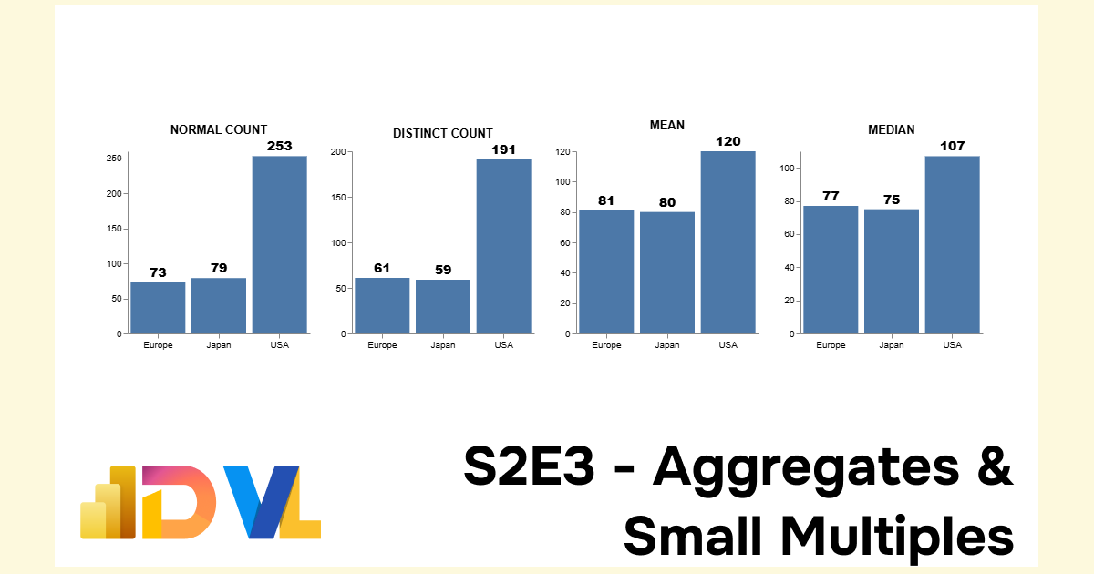
And now we begin to see our data outputs taking shape: Note: each aggregate result summarises effortlessly against the [Origin] field
| Origin | standard_count | distinct_count | mean_horsepower | median_horsepower |
|---|---|---|---|---|
| USA | 254 | 191 | 119.9 | 106 |
| Europe | 73 | 61 | 80.9 | 77 |
| Japan | 79 | 59 | 79.8 | 75 |
Step 3: Small Multiples
So far so good, and not a DAX measure in sight 🤓
What would be pretty cool now, is if we could separate our four aggregations into four separate charts, in the style of small multiples. It’s tantalisingly easy… follow me!
There are several ways to achieve the affect of small multiples using combinations of view layering and concatenations:
For ease and flexibility, I’ll showcase repeat here. But the PBIX 1 attached contains all varieties 🧙🏼♂️
I’ll write the before and after JSONs for comparison. The main difference is we wrap our mark and encoding block withing a spec block:
repeat and spec
1
2
3
4
{
  "repeat": [],
  "spec": { "mark":{}, "encoding":{} }
}
Pre-small multiples
1
2
3
4
5
6
7
8
9
10
11
12
13
14
15
16
17
18
19
20
21
22
23
24
25
26
27
{
  "data": {"url": "https://raw.githubusercontent.com/vega/vega/refs/heads/main/docs/data/cars.json"},
  "transform": [
    {
      "aggregate": [
        {"op": "count", "field": "Name", "as": "standard_count"},
        {"op": "distinct", "field": "Name", "as": "distinct_count"},
        {"op": "mean", "field": "Horsepower", "as": "mean_horsepower"},
        {"op": "median", "field": "Horsepower", "as": "median_horsepower"}
      ],
      "groupby": ["Origin"]
    }
  ],
   "title": {"text": "Aggregates and Facets", "anchor": "middle"},
  "width": 150,
  "mark": {"type": "bar"},
  "encoding": {
    "x": {
		"field": "Origin",
		"type": "nominal"
	},
    "y": {
		"field": "mean_horsepower",
		"type": "quantitative"
	}
  }
}
Post-small mulitples
1
2
3
4
5
6
7
8
9
10
11
12
13
14
15
16
17
18
19
20
21
22
23
24
25
26
27
28
29
30
31
32
33
34
35
36
37
38
39
40
41
42
43
44

{
  "data": {"url": "data/cars.json"},
  "transform": [
	// Our four aggregate transforms
    {
      "aggregate": [
        {"op": "count", "field": "Name", "as": "standard_count"},
        {"op": "distinct", "field": "Name", "as": "distinct_count"},
        {"op": "mean", "field": "Horsepower", "as": "mean_horsepower"},
        {"op": "median", "field": "Horsepower", "as": "median_horsepower"}
      ],
      "groupby": ["Origin"]
    }
  ],
  // start the repeat operation
  "repeat": [
    "standard_count",
    "distinct_count",
    "mean_horsepower",
    "median_horsepower"
  ],
  "spacing": 10,    // the spacing between charts
  "title": {"text": "Aggregates and Facets", "anchor": "middle"},
  "spec": {                             // wrap the mark properties in spec
    "width": 95,
    "height": 85,
    "mark": "bar",
    "encoding": {
      "x": {
        "field": "Origin",              // x-axis is unchange
        "sort": {"field": "Origin"},
        "axis": {"labels": true}
      },
      "y": {
        "field": {"repeat": "repeat"},  // y-axis uses the repeat fields instead of calculated fields
        "axis": {"labels": true},
        "type": "quantitative"
      },
    }
  },
  "resolve": {"scale": {"y": "shared"}} //
}
We now get this magical result:
Step 4: Finishing touches
We are close to perfection, we just want to add a splash of colour. We’ve been here before, just a simple "color": {"field": "Origin"} property in our encoding block.
Chef’s Kiss et voilà! 🧑🏽🍳
. . .
En Fin, Serafin
Thank you for staying to the end of the article… I hope you find it useful 😊. See you soon, and remember… #StayQueryous!🧙♂️🪄
PBIX 💾
🔗 Repo: Github Repo PBIX Treasure Trove

. . .
Footnotes
PBIX: Repo - Walkthrough Series ↩︎ ↩︎2