S2E4 - Join Aggregate Transform

Demystify Vega-Lite Examples in this step-by-step rebuild 🕊️🧙🏼‍♂️✨

Posted Apr 6, 2025 Updated Apr 6, 2025

Join Aggregate

By Imran Haq , PBI DataVizzle

7 min read

S2E4 - Join Aggregate Transform

💌 PBIX file available at the end of the article ¹ Enjoy!

Intro

Welcome to Season 2 of the Vega-Lite walkthrough series. In this season, we will go step-by-step through many of the Vega-Lite Examples - learning loads of techniques and tips along the way. Enjoy and welcome! 🕊️

Data

All data used in this series can be found in the Vega github repo:
Official Vega & Vega-Lite Data Source Repo

Dataset:

cars.json

Name	Origin	Horsepower	Year
chevrolet chevelle malibu	USA	130	1970-01-01
buick skylark 320	USA	165	1970-01-01
plymouth satellite	USA	150	1970-01-01
amc rebel sst	USA	150	1970-01-01

(Summarised & Aggregated)

Origin	Count	Distinct Count
USA	253	191
Europe	73	61
Japan	79	59

. . .

Concept

Here is the concept we will rebuild and better understand. The full script can be expanded below.

Important Note: Viewing Vega/Vega-Lite Outputs
When opening in the Vega Online Editor, remember to delete the raw path url before /data/. Examples:
Github pages:
• “data”: {“url”: “https://raw.githubusercontent.com/vega/vega/refs/heads/main/docs/data/stocks.csv”}
For online editor:
• “data”: {“url”: “data/stocks.csv}
For PowerBI:
• “data”: {“name”: “dataset”}

Reveal Vega-Lite Spec:

  
{
  "$schema": "https://vega.github.io/schema/vega-lite/v5.json",
  "description": "Multi-series line chart with labels and interactive highlight on hover.  We also set the selection's initial value to provide a better screenshot",
  "width": 600,
  "height": 300,
  /* when opening in the Vega Online Editor, remember to delete the raw path url before /data/ */
  /* • eg: for online editor | "data": {"url": "data/stocks.csv"} */
  /* • eg: for PowerBI | "data": {"name": "dataset"} */
  "data": {
    "name": "dataset"
  },
  // transforms
  "transform": [
    {
      /* we can add multiple aggregate operations */
      "aggregate": [
        {
          "op": "distinct",
          "field": "Name",
          "as": "distinct_count"
        },
        {
          "op": "count",
          "field": "__row_number__",
          "as": "normal_count"
        }
      ],
      "groupby": [
        "Origin"
      ]
    },
    {
      /* we can add multiple aggregate operations */
      "joinaggregate": [
        {
          "op": "sum",
          "field": "distinct_count",
          "as": "distinct_count_ja"
        },
        {
          "op": "sum",
          "field": "normal_count",
          "as": "normal_count_ja"
        }
      ],
      "groupby": []
    },
    {
      "calculate": "(datum.normal_count / datum.normal_count_ja)",
      "as": "normal_count_pct"
    },
    {
      "calculate": "(datum.distinct_count / datum.distinct_count_ja)",
      "as": "distinct_count_pct"
    }
  ],
  
  "hconcat": [
    {
      "title": "NORMAL COUNT",
      "width": 150,
      "layer": [
        {
          "mark": {
            "type": "bar",
            "strokeWidth": 0.8,
            "stroke": "black"
          }
        },
        {
          "mark": {
            "type": "text",
            "baseline": "middle",
            "fill": "black",
            "fontWeight": 900,
            "fontSize": 14
            //"dy": 20
          },
          "encoding": {
            "y": {
              "field": "normal_count_pct",
              "bandPosition": 0.5,
              "type": "quantitative"
            }
          }
        }
      ],
      "encoding": {
        "y": {
          "field": "normal_count_pct",
          "type": "quantitative",
          "aggregate": "sum",
          "stack": "normalize"
        },
        "order": {
          "field": "normal_count_pct",
          "sort": "descending"          
        },
        "color": {
          "field": "Origin",
          "type": "nominal",
          "scale": {
            "scheme":"pastel1"
          }
        },
        "text": {
          "field": "normal_count_pct",
          "type": "quantitative",
          "format": "0.1%"
        },
        "detail": {
          "field": "Origin"
        }
      }
    },
    {
      "title": "DISTINCT COUNT",
      "width": 150,
      "layer": [
        {
          "mark": {
            "type": "bar",
            "strokeWidth": 0.8,
            "stroke": "black"
          }
        },
        {
          "mark": {
            "type": "text",
            "baseline": "middle",
            "fill": "black",
            "fontWeight": 900,
            "fontSize": 14
            //"dy": 20
          },
          "encoding": {
            "y": {
              "field": "distinct_count_pct",
              "bandPosition": 0.5,
              "type": "quantitative"
            }
          }
        }
      ],
      "encoding": {
        "y": {
          "field": "distinct_count_pct",
          "type": "quantitative",
          "aggregate": "sum",
          "stack": "normalize"
        },
        "order": {
          "field": "distinct_count_pct",
          "sort": "descending"          
        },
        "color": {
          "field": "Origin",
          "type": "nominal",
          "scale": {
            "scheme":"pastel1"
          }
        },
        "text": {
          "field": "distinct_count_pct",
          "type": "quantitative",
          "format": "0.1%"
        },
        "detail": {
          "field": "Origin"
        }
      }
    }
  ]
}

. . .

Build

Step 1: What is the Join Aggregate Transformation?

It’s actually harder to explain than it is to show 🤓 - but I will try to do both and hope it makes sense. The easiest way to look at it is that Join Aggregate is similar to the Aggregate function. The BIG difference is that instead of transforming your dataset entirely, it takes the RESULT of your AGGREGATED dataset and JOINS it back onto your existing dataset.

For example: We take the original dataset…

Name	Origin	Horsepower	Year
chevrolet chevelle malibu	USA	130	1970-01-01
buick skylark 320	USA	165	1970-01-01
plymouth satellite	USA	150	1970-01-01
amc rebel sst	USA	150	1970-01-01

Then with Aggregate Transform, our dataset is transformed returning count and distinct count columns. The original dataset is transformed and summarised.

So Aggregate takes us from this…

  
{
      /* we can add multiple aggregate operations */
      "aggregate": [
        {
          "op": "distinct",
          "field": "Name",
          "as": "distinct_count"
        },
        {
          "op": "count",
          "field": "__row_number__",
          "as": "normal_count"
        }
      ],
      /* Note: Groupby field is necessary here*/
      "groupby": [
        "Origin"
      ]
    }

Origin	Count	Distinct Count
USA	253	191
Europe	73	61
Japan	79	59

…becomes this:

  
/* we can add multiple aggregate operations */
    {
      "aggregate": [
        {
          "op": "distinct",
          "field": "Name",
          "as": "distinct_count"
        },
        {
          "op": "count",
          "field": "__row_number__",
          "as": "normal_count"
        }
      ],
      /* Note: Groupby field is not needed as we need the grand total*/
      "groupby": []
    }

Total Count	Distinct Count
311	405

Due to the summarisation, we have lost the Origin field detail.

Note how this differs to Join Aggregate. Now we can summarise the grand totals and join the result back onto the original dataset, which gives us the following:

  
{
      /* we can add multiple aggregate operations */
      "joinaggregate": [
        {
          "op": "sum",
          "field": "distinct_count",
          "as": "distinct_count_ja"
        },
        {
          "op": "sum",
          "field": "normal_count",
          "as": "normal_count_ja"
        }
      ],
      "groupby": []
    }

Origin	Count	Total Count	Distinct Count	Total Distinct Count
USA	253	311	191	405
Europe	73	311	61	405
Japan	79	311	59	405

Step 2: How is this useful?

This is the key question. When and why would we use this? There are several use cases, but the most useful one I have found is calculation the percentage of the total.

Returning to our Join Aggregate dataset, we have our numerator (counts) and with join aggregate transforms we now have our denominator (total counts). With these two fields, we can now determine each rows value and what the percentage is of the grand total.

Step 3: Derive the Percentage (of Total)

We’ve been here before, this is our bread 🍞 and butter 🧈 calculate transform:

  
"transform": [{
  "calculate": " ( datum.numerator / datum.denominator )", "as": "percentage_field"
}] 

In context, we will reuse the results of our previous Aggregate and Join Aggregate transforms:

  
"transforms": [
    {
      "calculate": "(datum.normal_count / datum.normal_count_ja)",
      "as": "normal_count_pct"
    },
    {
      "calculate": "(datum.distinct_count / datum.distinct_count_ja)",
      "as": "distinct_count_pct"
    }
]

(separated for emphasis)

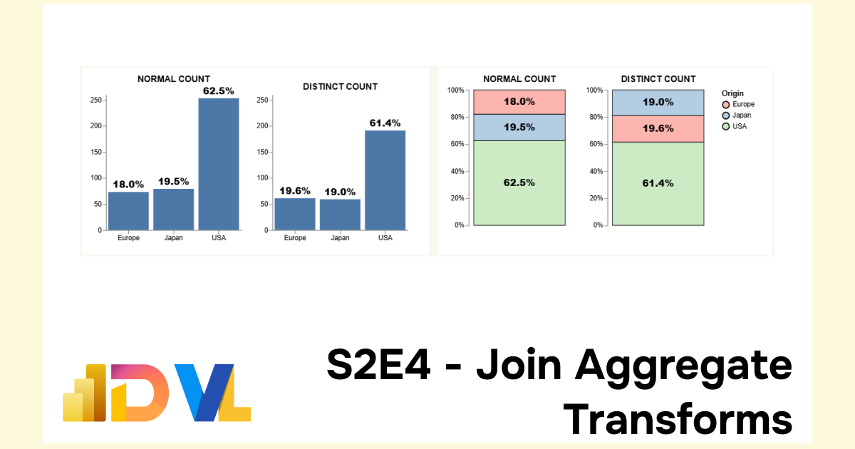
Origin	Count	Total Count	Normal Count PCT
USA	253	311	0.624
Europe	73	311	0.180
Japan	79	311	0.195

Origin	Distinct	Total Distinct Count	Distinct Count PCT
USA	191	405	0.614
Europe	61	405	0.196
Japan	59	405	0.189

Step 4: Create our DataViz

This is our moment to piece everything together. Noone can stop this freight train 🚄

. . .

En Fin, Serafin

Thank you for staying to the end of the article… I hope you find it useful 😊. See you soon, and remember… #StayQueryous!🧙‍♂️🪄

PBIX 💾

🔗 Repo: Github Repo PBIX Treasure Trove

. . .

Footnotes

PBIX: Repo - Walkthrough Series ↩︎

Season-2, Charts, DataViz, Deneb, Vega-Lite, Walkthrough

season2 walkthrough

This post is licensed under CC BY 4.0 by the author.

Intro

Data

Dataset:

(Summarised & Aggregated)

Concept

Build

Step 1: What is the Join Aggregate Transformation?

Step 2: How is this useful?

Step 3: Derive the Percentage (of Total)

(separated for emphasis)

Step 4: Create our DataViz

En Fin, Serafin

PBIX 💾

Footnotes

Trending Tags